

5 Ways to Hide Data in Excel
5 Ways to Hide Data in Excel: Are you for ways to place some secret text or data in Excel. Well here are few awesome excel tricks for you… You can watch the step by step video or continue reading the blog.
Method 1: Using Freeze panes option to hide excel data
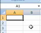
Step 1: Go to cell A100 and type or paste the data which you want to hide.

Step 2: Now Go back to cell A1
Step 3: Zoom to 20%

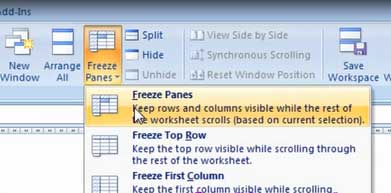
Step 4: Now carefully Place the cursor in the cell A100 and click on freeze panes option on the view tab.
Step 5: Now Go back to call A1 again and Zoom to 100%
Step 6: Now if you scroll the sheet you could notice that the sheet doesn’t scroll and the data in and below the cell A100 is not displayed.
Step 7: You may protect the sheet with a password to prevent the user from unfreezing the panes.
Watch the video of (5 Ways to Hide Data in Excel) for more accurate steps and details
Method 2: Overlapping an image that looks like worksheet cells to hide excel data
Step 1: Select empty cells as same as the size of the data.

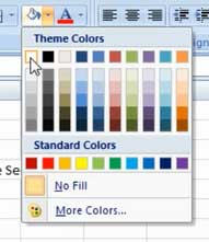
Step 2: Then fill it with white background color
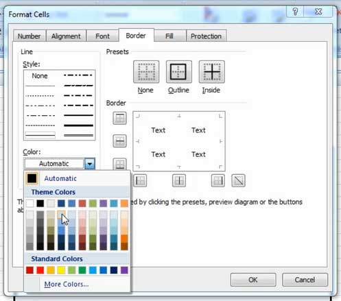
Step 3: Then Apply ‘Dark Blue, Text 2, Lighter 80%’ for the cell’s border color.
Step 4: With the cells still selected, go to the home tab then–> paste–>as picture–>copy as picture.

Step 5: Now paste the copied image.
Step 6: Then drag it over the data that you want to hide.
Step 7: Make sure that you align the image exactly on the cell borders… So that it looks like empty cells…
Watch the video of (5 Ways to Hide Data in Excel) for more accurate steps and details
Method 3: Hiding data with color
You can use the font color to hide the text. You can set the font color as same as the cells background color. For example: If the cells background color is white then you should also set the font color to white. This makes the text or data invisible.
Method 4: Hiding behind a textbox, picture, clipart or a chart
- Hiding behind a textbox
- Hiding behind a picture or a image or a clipart
Method 5: Hiding behind a chart
- Hiding rows, columns, entire worksheet or entire workbook
- Hiding rows and columns
- Hiding rows entire worksheet
Watch the video for more accurate steps and details. I hope that the tutorial was interesting. Catch you with another interesting tutorial soon. Please leave your doubts and questions in the comments below.
Similar Tutorials, Excel News & Articles:
Huge List of Free Excel learning sites
Excel Tutorial VBA Macros – How to create a number chart 1 to 100 using Excel macro
18 Advanced Excel Tips and Tricks, Excel Secrets you don’t know
How to record excel macro using macro recorder Best example
Excel vba Userform tutorial – How to create number series using Userform
- MS Word Shortcut Keys PDF - October 13, 2024
- What is MS Word and its Features PDF - October 10, 2024
- 10 Free Word Templates for Every Need - October 10, 2024